Evaluating the Break Even Period of Our Solar Battery
A little while ago, I wrote a post on Monitoring Solar Generation stats with InfluxDB, Telegraf and Soliscloud.
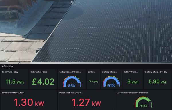
Since then, one of the things that I've been working on is a Grafana dashboard to track our path towards break-even: that is, when the system has "saved" us enough that it's paid the costs of purchase and install.
As well as charting the break-even path of the system as a whole, the dashboard also calculates individual break-even for the battery. Because battery storage is an optional part of a solar install, I thought it'd be interesting to calculate what kind of difference it was making versus the cost of adding it.
I actually sort of wish that I hadn't, because the thing that's stood out to me is just how long the battery's break-even period actually is.
In this post, I'll talk about how I'm calculating amortisation stats, what I'm seeing, possible causes and what I think it all means.
Defining Battery Benefit
In order to calculate the total value that the battery has unlocked, we first need to be able to define how the battery releases value.
The flow of energy through the system is pretty simple:
- Solar panels generate electricity
- Power required for current household demand flows to the household
- The remainder is either exported or used to charge the battery
Number 3 isn't actually an either/or: there will be times when energy is going to the battery and being exported:
It can be quite tempting to view the battery's energy output as pure financial value, giving a nice endorphin hit when you see it delivering nkWh a day (or, contributing to a high percentage of your daily consumption being locally served). However, that's only part of the financial picture because we also need to account for lost opportunity cost.
If the battery wasn't present, the energy charged into it would have instead been exported (because there wasn't sufficient household consumption at that time of day to sup those particular electrons) and we'd have received an export payment for it.
Just like any other profit margin calculation we need both an input and an output:
-
input value: To account for the lost export revenue, this is defined by the export tariff (currently,£0.15/kWh) at time of charging. -
output value: The cost of a discharged kWh (at time of use) if we'd instead had to import it from the grid (I'm on Octopus Agile so the price varies every 30 minutes).
With those two values, calculating savings is simple:
   output_value
 - input_value
   ==============
   savings_value

# For example: 1kWh

stored @ £0.15/kWh
discharged @ £0.35/kWh
========================
£0.35 - £0.15 = £0.20
========================

Savings: £0.20
I created downsampling jobs which calculate and store these statistics periodically so that I don't need to include these calculations in the queries that I write. The jobs uses the logic described above, pulling in Octopus pricing information along with our battery charge and discharge figures.
downsample_battery_financial_value:
    name: "Downsample Solar financial value"
    influx: home1x
    period: 2880
    query: >
       pricing = from(bucket: "Systemstats/autogen")
            |> range(start: v.timeRangeStart, stop: v.timeRangeStop)
            |> filter(fn: (r) => r._measurement == "octopus_pricing"
                and r._field == "cost_inc_vat"
                and r.charge_type == "usage-charge"
                and r.tariff_direction != "EXPORT"
                )
            |> filter(fn: (r) => r.payment_method == "None")
            |> aggregateWindow(every: 30m, fn: max)
            |> keep(columns: ["_time","_field","_value"])

        battery_activity = from(bucket: "Systemstats/autogen")
            |> range(start: v.timeRangeStart)
            |> filter(fn: (r) => r._measurement == "solar_inverter"
                and (r._field == "batteryChargeToday"
                     or r._field == "batterySupplyToday"
                ))
            |> aggregateWindow(every: 30m, fn: max)
            |> difference(nonNegative: true)
            |> keep(columns: ["_time","_field","_value"])
            |> pivot(rowKey: ["_time"], columnKey: ["_field"], valueColumn: "_value")

        usage_values = join(tables: {price: pricing, activity: battery_activity}, on: ["_time"])
        |> map (fn: (r) => ({
          _time: r._time,
          battery_stored : r.batteryChargeToday * r._value,
          battery_discharged : r.batterySupplyToday * r._value,
          _measurement: "solar_value"
        }))

        batteryCharge = usage_values
              |> map(fn: (r) => ({
                _time: r._time,
                _measurement: r._measurement,
                _field: "battery_stored",
                _value: r.battery_stored
              }))

        batteryDischarge = usage_values
              |> map(fn: (r) => ({
                _time: r._time,
                _measurement: r._measurement,
                _field: "battery_supplied",
                _value: r.battery_discharged
              }))

        union(tables: [batteryDischarge, batteryCharge])

    aggregates:
        copy:

    output_influx:
        - influx: home2xreal
    output_bucket: Systemstats/rp_720d
A second similar job calculates the potential export value (stored in field battery_stored_value_if_exported).
Calculating The Path to Break Even
With a record of accrued savings available, calculating the amount left before break-even is simple, we subtract accrued savings from the amount that we paid to buy and install the battery (the capital cost).
  battery_cost
- sum(savings_value)
  ===================
  remaining_cost
We can also generate a projection of how long it'll take to break even, by dividing remaining_cost with the daily average sum() of savings_value:
battery_cost = <redacted>

// Fetch the monetary value of energy supplied by the battery
// calculate the per day total
supply = from(bucket: "Systemstats/rp_720d")
  |> range(start: v.timeRangeStart, stop: v.timeRangeStop)
  |> filter(fn: (r) => r["_measurement"] == "solar_value")
  |> filter(fn: (r) => r["_field"] == "battery_supplied")
  |> aggregateWindow(every: 1d, fn: sum, createEmpty: false)
  |> map(fn: (r) => ({
      _time: r._time,
      _field: r._field,
      _value: r._value / 100.0
  }))


// Fetch the potential monetary value of energy if it had been
// exported rather than stored
export_val = from(bucket: "Systemstats/rp_720d")
  |> range(start: v.timeRangeStart, stop: v.timeRangeStop)
  |> filter(fn: (r) => r["_measurement"] == "solar_value")
  |> filter(fn: (r) => r["_field"] == "battery_stored_value_if_exported")
  |> aggregateWindow(every: 1d, fn: sum, createEmpty: false)
  |> map(fn: (r) => ({
      _time: r._time,
      _field: r._field,
      _value: r._value / 100.0
  }))

// Subtract the export value from the supply value to
// calculate savings_value
//
savings_value = join(tables: {supply: supply, export: export_val}, on: ["_time"])
  |> map(fn: (r) => ({ r with
     _value: r._value_supply - r._value_export
  }))

// Calculate the mean daily saving
mean_savings = savings_value
  |> mean()
  |> findRecord(
        fn: (key) => true,
        idx: 0,
  )

// Sum the savings accrued since the system
// was installed and substract from the cost
// divide the remainder by the avg daily savings
// the result is an estimation of the number of
// days until break even
savings_value
  |> sum()
  // Subtract the savings from the capital cost
  // to calculate "remainining_cost"
  // and then divide the remainder by mean(savings_value)
  |> map(fn: (r) => ({ r with
     _value: (battery_cost - r._value) / mean_savings._value
  }))
Unexpected Break Even Period
Ever since we began looking at Solar, I've thought of a battery as something which unlocks additional value.
So, it took me by surprise to see just how long the battery's projected break-even period was in comparison to the system as a whole.

This is about 30% more than the break-even period for the whole system (the cost of which includes not just the panels but scaffolding and labour etc).

12 years is longer than the battery's warrantied life, raising the possibility that it might never actually be able to deliver enough savings to break even!
Skewed Results
That's not great, but things are still actually worse than they seem: the 12.6 year figure is heavily skewed and should probably be a lot higher.
The problem is, there's a long delay between install and receiving the certificates and paperwork that are necessary to set up an export tariff. Without that export tariff, no-one's paying you for exported energy, giving every kWh exported a financial value of... diddly squat.
So, for more than half the time that the data covers, the sum that we've actually been doing is
  output_value
- 0.00
  =============
  savings_value
In other words, every kWh discharged from the battery during that period is counted as pure profit because it would have been worthless if exported to the grid.
This gave the overall savings_value a big headstart:

It's quite obvious where in the chart the export tariff came into effect: aside from one bumper day, the savings value dropped right off (we'll come back to that negative day in a bit).
Why??
Electricity Prices
The first contributing factor is the market value of each kWh.
Whilst this is, undoubtedly, a nice problem to have, the poor battery savings rate is partially driven by generous export values.
On our current tariffs:
- Export has a flat rate of
£0.15/kWh - Import has an average rate of
£0.21/kWh(maxing out at£0.47/kWh)
The export value is a very generous 71% of the average import value. This isn't a bad thing overall, but, because savings are based on a delta of import & export, it does limit the potential savings that the battery can unlock.
This is mitigated a little by the fact that (by design) the battery tends to be discharged at peak times, when import prices are higher.
The following Flux query extracts daily pricing during peak hours (defined as 16:00-20:00)
import "date"

from(bucket: "Systemstats")
  |> range(start: v.timeRangeStart, stop: v.timeRangeStop)
  |> filter(fn: (r) => r._measurement == "octopus_pricing")
  |> filter(fn: (r) => r._field == "cost_inc_vat")
  |> filter(fn: (r) => r.charge_type == "usage-charge"
                    and r.tariff_direction != "EXPORT"
                    and r.tariff_code == "E-1R-AGILE-FLEX-22-11-25-A"
                    and r.payment_method == "None"
                )
  |> keep(columns: ["_time", "_field", "_value"])
  // Filter to only return results from peak hours
  // times are in UTC, but the UK is in UTC+1 atm, so 16-20 becomes 15-9
  |> filter(fn: (r) => contains(value: date.hour(t: r._time), set: [15,16,17,18,19]))
  // Convert from pence to pounds for Grafanas benefit
  |> map(fn: (r) => ({r with _value:  r._value / 100.0}))

If we append a line to the query to calculate the overall mean:
|> mean()
We can see that the average peak-hour unit price on Octopus Agile is currently £0.268 per kWh (meaning that the export value is 56% of the average peak hours import price).
So, on average, the battery will save £0.118/kWh during peak hours.
That's not bad, but it takes a lot of 11.8 pences to make up the capital cost of the battery. In fact, we'd need tens of mega-watt-hours of peak-time usage, translating to a long break-even period.
Average Battery Charge Level
It should go without saying that, the more energy we cram into the battery, the more that we stand to save.
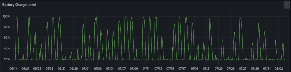
We've got a 6kWh battery and, even in the short time that we've had it, I've occasionally wished that I'd added an extra cell.
But, querying the average maximum daily charge level shows that, on average, the maximum charge level of the battery is 72.7%
from(bucket: "Systemstats/rp_720d")
  |> range(start: v.timeRangeStart, stop: v.timeRangeStop)
  |> filter(fn: (r) => r["_measurement"] == "solar_inverter")
  |> filter(fn: (r) => r["_field"] == "batteryPowerPerc")
  |> keep(columns: ["_time", "_field", "_value"])
  |> aggregateWindow(every: 1d, fn: max, createEmpty: false)
  |> mean()

So, most of the time, we're not actually making full use of the capacity that we have.
There are, of course, days where we fill the battery to the brim, but the average is persistently lower than that, even in these summer months (such as they are)

This means that, on average, the battery has 4.38kWh stored and so (at 11.8 pence) can unlock a maximum saving of £0.52/day.
Without the head start that not having an export tariff gave, at £0.52 a day, we'd be looking at decades until break-even.
Adjusting the Break-Even Projections
In fact, it's possible for us to account for that headstart by adjusting the averaging performed in the battery break even query so that those higher figures are normalised down (I've used the median value since the export tariff came online)
mean_savings = savings_figures
  // If the value is greater than £1.50
  // normalise it to the median of 0.12
  |> map(fn: (r) => ({ r with
     _value: if r._value > 1.5
        then 0.12
        else r._value
  }))
  |> mean()
  |> findRecord(
        fn: (key) => true,
        idx: 0,
  )
The result really doesn't look too peachy:

If we adjust the System break-even calculation query so that is also normalises battery savings, the resulting projection is 30% longer than the original system break-even projection
daily_avg = from(bucket: "Systemstats/rp_720d")
  |> range(start: v.timeRangeStart, stop: v.timeRangeStop)
  |> filter(fn: (r) => r["_measurement"] == "solar_value")
  |> filter(fn: (r) => r["_field"] == "solar_value_pence" or r["_field"] == "battery_supplied")
  |> aggregateWindow(every: 1d, fn: sum, createEmpty: false)
  |> map(fn: (r) => ({r with _value: r._value / 100.0}))
  |> pivot(rowKey: ["_time"], columnKey: ["_field"], valueColumn: "_value")
  // Deduct battery savings from the solar value
  // then normalise battery supply values to remove the
  // headstart figures
  |> map(fn: (r) => ({ r with
     _value: r.solar_value_pence - r.battery_supplied,
     battery_normalised: if r.battery_supplied > 1.5
        then 0.12
        else r.battery_supplied
  }))
  // Add the battery supply value back on
  |> map(fn: (r) => ({
     _value: r._value + r.battery_normalised,
     _field: "solar_value_pence",
     _time: r._time
  }))
  |> mean()
  |> findRecord(
        fn: (key) => true,
        idx: 0,
  )
  // snip amortisation calculations

Proportionally, it's a big jump but... I actually expected it to be much worse.
Usage
Another contributing factor is the level of our overall electricity consumption during those valuable peak hours. Because we're on a 30-minute tariff, 1kWh saved at 10pm simply isn't as valuable as the same amount saved at 6pm.
The following query shows peak consumption per-day (fair warning: I'd had a few Southern Comforts when I wrote this)
import "date"

from(bucket: "Systemstats")
  |> range(start: v.timeRangeStart, stop: v.timeRangeStop)
  |> filter(fn: (r) => r._measurement == "solar_inverter")
  |> filter(fn: (r) => r._field == "consumptionToday")
  |> keep(columns: ["_time", "_field", "_value"])
  |> filter(fn: (r) => contains(value: date.hour(t: r._time), set: [15,16,17,18,19]))
  // Group by day
  |> map(fn: (r) => ({r with
     day: string(v:date.month(t: r._time)) + string(v: date.monthDay(t: r._time))
     }))
  |> group(columns: ["day"])
  // Get the Min and max per group
  // preserve the final timestamp
  |> reduce(fn: (r, accumulator) => ({
      _time: r._time,
      min: if r._value < accumulator.min then r._value else accumulator.min,
      max: if r._value > accumulator.max then r._value else accumulator.max,
      }),
      identity: {
        _time: 1970-01-01,
        min: 4000.0,
        max: 0.0
        }
  )
  // Subtract min from max to get the consumption for that period
  |> map(fn: (r) => ({
    _time: r._time,
    _field: "consumption",
    _value: r.max - r.min
  }))
At time of writing, the resulting graph looks like this
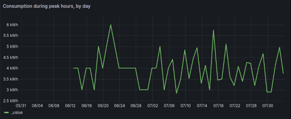
If we adjust the query to calculate the overall mean:
|> mean()
We find that on average, we consume 3.96 kWh during peak hours.
Negative Savings
Because they drag averages down, negative daily savings can have a significant effect on the break-even period calculations.
In the graph of daily battery savings that we looked at earlier, there was a day which reported negative savings:
The stats report that the battery saving for 29-30 of July was -£0.114: we effectively paid 11 pence because we've got a battery!
There are two main ways that savings can turn negative
- High usage during an Octopus Plunge Pricing event (where import prices are negative)
- Not enough "value" being drawn during discharge (whether due to low consumption or lower import prices)
Plunge pricing events don't generally happen during peak times, so (whilst possible) it's far less likely as a factor. The Octopus pricing graphs for that day confirm that, whilst it was a cheap day, prices didn't go negative:

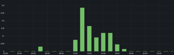
There was a period where energy was particularly cheap, but there's no corresponding household usage to suggest we might have drawn a large amount of energy from the battery:

In fact, consumption was pretty much flat that day (we must not have used the oven in the evening).
If we look at the "savings" of that day in more detail, we can see that they went heavily negative in the morning:

Between the two graphs, we can see that negative period doesn't coincide with household usage, but instead represents the export value of the power being charged into the battery:
from(bucket: "Systemstats/rp_720d")
  |> range(start: v.timeRangeStart, stop: v.timeRangeStop)
  |> filter(fn: (r) => r["_measurement"] == "solar_value")
  |> filter(fn: (r) => r["_field"] == "battery_stored_value_if_exported")
  |> aggregateWindow(every: 1h, fn: sum, createEmpty: false)
  |> keep(columns: ["_time", "_field", "_value"])
  |> map(fn: (r) => ({r with _value: r._value / 100.0}))
Even non-negative days have a profile with a negative period like the one shown above: in effect, we incur a "cost" whilst charging, in the hope that the value of usage later in the day will exceeded the sacrificed export cost.
The problem on this particular day was that the battery got a good charge, but too little energy was consumed during peak-hours, meaning that the import savings didn't outweigh the lost opportunity cost of the initial energy investment.
System Sizing
Low savings can also be driven by an imbalance in terms of system sizing.
I've got 6 kWh of battery capacity, and 3.8 kWp of panels on the roof. That difference wasn't entirely by choice (and I'm still a tad salty about it).
When the surveyor visited, he took measurements and said we could only fit 4 panels on each roof. So, instead of the 10 panels that I'd planned for, we installed 8 (the loss of those extra panels freed up funds for an extra pack in the battery).
On install day, though, the roofer arrived and asked if it was OK to install some of the panels portrait because it made fitting the rails easier. With the panels portrait, another 2 panels could easily have fit on each roof.... grrrr.
Annoying as that was, the truth is that the battery is probably sized about right for our usage.
As we saw above:
- We're storing an average of
4.38 kWhper day. - We're drawing an average of
3.96 kWhof that during peak hours
On average, peak hours consume about 90% of the energy that we store into the battery, so it's doing exactly what it's supposed to and insulating us from peak-time pricing.
Although there are exceptions, most nights the battery continues covering our usage into the small hours of the next day:
It's true that (assuming we could charge it) a larger battery would cover usage further into the next day, but the cost/benefit of that probably doesn't make sense either: by around 10pm the import cost is often close to or lower than the export value, increasing the likelihood of our battery savings turning negative.
Weather Patterns
There's no other way to say it really: the weather has been crap this summer, with the UK "enjoying" an unseasonably cloudy and wet July.
However, whilst that delays break-even of the whole system, it has a fairly limited impact on the break-even performance of the battery: we're generally still storing more than we draw during the hours that really matter.
When Winter comes around though, things might shift a little:
- The peak per-unit cost will generally be higher than in Summer, improving "savings"
- The days will be shorter and the weather worse, so less energy will be stored to the battery, reducing "savings"
The unknown is whether 1. will outweigh 2.
I suspect that it's unlikely to - if nothing else, it also raises the costs incurred if the battery does run flat before peak hours are complete.
It's also not certain that prices in Winter will be much higher than now - prices are still trending down from the spike that happened as a result of Russia invading Ukraine.
System Break-Even Without The Battery
So, there's an obvious question here: what would solar value and break-even look like if we hadn't installed the battery in the first place?
To approximate that, we first need to look at the value of the electricity generated, subtracting the battery supply value and re-adding it's equivalent export value:
from(bucket: "Systemstats/rp_720d")
  |> range(start: v.timeRangeStart, stop: v.timeRangeStop)
  |> filter(fn: (r) => r["_measurement"] == "solar_value")
  |> filter(fn: (r) => r["_field"] == "solar_value_pence"
                    or r["_field"] == "export_value_pence"
                    or r["_field"] == "battery_supplied"
                    or r["_field"] == "battery_stored_value_if_exported"

  )
  // Calculate the value as follows
  //
  // Sum solar_value annd export_value
  // Subtract the value supplied by the battery
  // because it's included in solar_value_pence and
  // without storage we'd have instead paid that price
  // Add the export values instead
  |> pivot(rowKey: ["_time"], columnKey: ["_field"], valueColumn: "_value")
  |> map(fn: (r) => {
    // export_value_pence doesn't exist on earlier records
    val = if exists r.export_value_pence
      then (r.solar_value_pence + r.export_value_pence + r.battery_stored_value_if_exported) - r.battery_supplied
      else (r.solar_value_pence + r.battery_stored_value_if_exported) - r.battery_supplied
    return {
     _time: r._time,
     _field: "pence",
     _value: val / 100.0
  }})
  |> aggregateWindow(every: 1d, fn: sum, createEmpty: false)
  |> sum()

This value is about £90 less than the value for our actual system: after all, the battery is providing some benefit, just not enough to outweigh its purchase price.
Without the battery, the install cost would also have been lower, so we need to re-run the amortisation query with a couple of changes
-
install_costis now the system install cost minus the invoiced cost of the battery - Daily averages are calculated using the battery-less solar value sums used in the query above
The query looks like this
// install cost is capital cost minus the cost
// of the battery
install_cost = <redacted>

daily_savings = from(bucket: "Systemstats/rp_720d")
  |> range(start: v.timeRangeStart, stop: v.timeRangeStop)
  |> filter(fn: (r) => r["_measurement"] == "solar_value")
  |> filter(fn: (r) => r["_field"] == "solar_value_pence"
                    or r["_field"] == "export_value_pence"
                    or r["_field"] == "battery_supplied"
                    or r["_field"] == "battery_stored_value_if_exported"

  )
  // Calculate the value as follows
  //
  // Sum solar_value annd export_value
  // Subtract the value supplied by the battery
  // because it's included in solar_value_pence and
  // without storage we'd have instead paid that price
  // Add the export values instead
  |> pivot(rowKey: ["_time"], columnKey: ["_field"], valueColumn: "_value")
  |> map(fn: (r) => {
    // export_value_pence doesn't exist on earlier records
    val = if exists r.export_value_pence
      then (r.solar_value_pence + r.export_value_pence + r.battery_stored_value_if_exported) - r.battery_supplied
      else (r.solar_value_pence + r.battery_stored_value_if_exported) - r.battery_supplied
    return {
     _time: r._time,
     _field: "pence",
     _value: val / 100.0
  }})
  |> aggregateWindow(every: 1d, fn: sum, createEmpty: false)


daily_avg = daily_savings
  |> aggregateWindow(every: 1d, fn: sum, createEmpty: false)
  |> keep(columns: ["_field", "_time", "_value"])
  |> mean()
  |> findRecord(
        fn: (key) => true,
        idx: 0,
    )

// Sum up the unlocked savings so far
// subtract that from the capital cost
// and divide the remainder by the daily average
daily_savings
  |> keep(columns: ["_field", "_value"])
  |> sum()
  |> map(fn: (r) => ({r with
     _value: (install_cost - r._value) / daily_avg._value
  }))
  |> yield(name: "remaining")
The result is that the remaining break-even period is about 16% shorter than that reported for the real system (and about 36% shorter than the estimate using the adjusted stats).

In practice, the break-even period would probably be even shorter because there are things that we've still not accounted for:
- Not having a battery means a less complex install, reducing labour costs
- A cheaper inverter could have been used
Both of these mean that install costs would likely have been lower, in turn reducing the break-even period even further.
Why This Matters
We've spent our money and, for better or worse, have a battery - so it's tempting to think that the figures above are moot because it's too late to change anything.
The reason that they matter, though, is because they can help inform how we act in future.
I had previously assumed that - at some point - we'd probably add an extra pack to the battery. On the face of it, though, it doesn't look like this would make financial sense even if we were regularly filling the current battery.
Despite the higher cost (because scaffolding), if we were going to expand the system, the more financially sensible answer would almost certainly be to add panels or some other form of generation (helping serve higher spikes in demand as well as driving up export revenue). Even then, though, the short-term gains would probably be marginal.
Mitigating
Given that we've already got the battery, there are, perhaps, other options that could be pursued in order to try and improve the break-even time.
Solar isn't the only way that a battery can be charged: it's also possible (if a bit fiddly with some inverters) to charge from the mains.
So, instead of storing energy that we could have been paid £0.15 to export, we can instead buy in and store when import prices are low in order to try and achieve a bigger saving.
To help assess the feasibility of this, we can check the minimum non-peak price per day.
We do this by taking our earlier peak-hour pricing and adjusting the time check. We also need to allow time for the battery to charge, so the query needs to also exclude a couple of hours prior to peak
import "date"

from(bucket: "Systemstats")
  |> range(start: v.timeRangeStart, stop: v.timeRangeStop)
  |> filter(fn: (r) => r._measurement == "octopus_pricing")
  |> filter(fn: (r) => r._field == "cost_inc_vat")
  |> filter(fn: (r) => r.charge_type == "usage-charge"
                    and r.tariff_direction != "EXPORT"
                    and r.tariff_code == "E-1R-AGILE-FLEX-22-11-25-A"
                    and r.payment_method == "None"
                )
  |> keep(columns: ["_time", "_field", "_value"])
   // Filter to only return results from outside
   // times are in UTC, but the UK is in UTC+1 atm, so 16-20 becomes 15-9
  |> filter(fn: (r) => not contains(value: date.hour(t: r._time), set: [13,14,15,16,17,18,19]))
  // Convert from pence to pounds for Grafanas benefit
  |> map(fn: (r) => ({r with _value:  r._value / 100.0}))
  |> aggregateWindow(every: 1d, fn: min)
The hours after peak aren't excluded, because we could conceivably use those to charge the battery ready for the next day.

(The 16th and 17th were Plunge Pricing days because of excess wind in NL and BE)
Although there are exceptions, the vast majority of days see periods with import prices that are lower than the export value.
If we calculate the average (plunge pricing is rare, so I've excluded those days)
|> filter(fn: (r) => r._value > 0.0)
|> mean()
We can see that, on average, the minimum daily price is 12.7p kWh.
So, by charging from the mains, we could increase our average per-kWh saving by 20%!
The problem is, that's still actually only a saving of 14.1p/kWh or (at our average of 4.38kWh charge) £0.62/day. The increased saving shaves a good chunk off that battery's break-even period, but it's still decades out.
Octopus Agile prices change every 30 minutes (and are known up to 24hrs in advance), so we could perhaps take it a step further and adopt more of a micro-trade type approach: charging and discharging a little as prices fluctuate throughout the day

The problem is, we'd then have to think much harder about the resulting wear & tear on the battery: it would almost certainly shorten the serviceable lifetime and so might still never manage to breakeven.
Adjusting Time Of Use
Energy stored in the battery is most valuable during peak hours. So, one option might be to adjust settings on the inverter so that it can only be discharged during those hours.
This would ensure that each kWh is "exchanged" for the highest possible price, with any charge left in the battery after peak hours being retained until peak the next day.
On cloudy days, this probably wouldn't lead to much difference. However, on sunnier days, we may see the battery retain increasingly higher charge levels, ultimately leading to more energy being exported (decreasing the system's overall payback time).
I don't know how much this would help in practice, but, it certainly seems worth experimenting with.
Conclusion
When I was planning the system's install, I was certain that having a battery made sense: After all, it doesn't make sense to export a kWh only to have to later buy it back at a higher price.
The problem is, the market price of solar batteries confounds that logic. Although costs have dropped significantly over the years, the capital cost of batteries is still high enough that (for our use case, at least) it'll not unlock enough savings to pay for itself.
Years back, I did some research into Premium Unleaded: it provides better fuel economy (mpg), but the additional cost per litre still makes it the more expensive option per mile. I've been reminded, quite heavily, of that whilst exploring these figures.
My battery break-even stats currently report battery break-even in 12.6 years, but that's the result of (temporary) statistical magic: delays in getting an export tariff set up meant that we enjoyed an extended period of pure profit (on paper at least). Real-terms savings are much lower, and the adjusted break even projections show that reported break-even time will extend significantly as daily-average calculations regress to the mean.
At current prices and usage, it looks as though it will take decades for the battery to pay for itself.
That the overall system, even with the adjusted figures, looks set to break-even in a little over a decade, really is testament to how much benefit the panels bring, managing to offset the lackadaisical battery savings.
Complicating Factors
It's worth noting that the calculations have been performed in a period where energy prices are still high as a result of Russia going full twat. I can only imagine what the break-even figures might have looked like with the prices we were enjoying before Putin's bloody folly.
Conversely, I've also not accounted for inflation: so long as my wages (and export values) eventually catch up, inflation is effectively degrading the value of the install "debt". With the world (and particularly the UK) very badly out of whack, though, the impact of future inflation is very hard to account for, so I haven't attempted to do so.
It's Not All Negative
It would be very easy to read this post and conclude that buying a solar battery doesn't make sense and from a purely financial perspective, that's probably true.
It does seem worth noting, however, that there is often more to these sort of decisions than finance maths.
Installing a solar battery is a hedge, made against energy prices shifting heavily in the future - whether a collapse in export value or a spike in import costs.
To use a more familiar analogy:
- It doesn't make financial sense to overpay on a low-interest mortgage instead of paying into a higher interest savings account (which can later be used to pay slightly more of the mortgage down).
- Many, though, find it gives psychological comfort to overpay their mortgage for the piece of mind that the debt is reduced in case something happens in future.
The same is probably true of a solar battery, it might not be paying for itself now, but that doesn't mean that it won't do so in the future (and if such a need arises, the cost of an install then will likely have increased proportionally).
As well as reducing monthly bills a little, there's also something to be said for knowing the units of energy that you're burning came from solar and not fossil fuels.
But, that's still a very different choice to purchasing a battery with the expectation that it'll save you money overall, because there's a non-negligible chance that it won't.
If I had a do-over
Based on these figures, I'm not sure that I would install a battery if I were doing this all over again. In fact, if an expensive repair were to arise, I'm not even sure that I wouldn't have it removed instead.
Whilst the battery does lead to a small reduction in monthly electricity bill, it's looks like it's still likely to be a net loss.
With the benefit of hindsight, the capital cost would have provided better returns sat in a savings account. In fact, given the annual return is less than 1%, the capital would even have been better placed in a bog-standard current account.