Collecting Octopus Energy Pricing and Consumption with Telegraf

As an energy supplier, Octopus Energy are pretty much unique (at least within the UK energy market), not least because they expose an easily accessible API allowing customers to easily fetch consumption and pricing details.

Like many others, I'm on Octopus Agile, so being able to collect past and future pricing information is particularly useful because that information enables us to try and shift load to when import rates are most favourable.

At times, this can be incredibly beneficial: for example, at time of first writing, the rates were negative, so we were actually getting paid (albeit a small amount) for the energy that we were consuming.

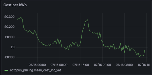
The next day's prices are published daily at around 4pm every day, allowing some manner of planning ahead (more plunge pricing tomorrow, yay!):

For those who want to build automations, there's an excellent integration for HomeAssistant, however, I spend more of my time in Grafana/InfluxDB than HomeAssistant so I also wanted Telegraf to be able to fetch this information.

In this post, I'll detail how to set up my Octopus Energy exec plugin for Telegraf and will also provide some examples of how I've started using that data within Grafana.

---

Dependencies

The plugin is a small python script, requiring the following

• Python 3
• The requests module (pip install requests)

---

Account Information

In order to fetch consumption information, the plugin needs to use an API key to authenticate with Octopus's API. It also needs to be able to figure out what meters you have and what tariff each is associated with, so it needs your account number.

Finding the necessary details is simple:

Log into https://octopus.energy and in the top left corner of the main dashboard will be your name followed by your account number

The account number should consist of a letter followed by a dash and some other characters.

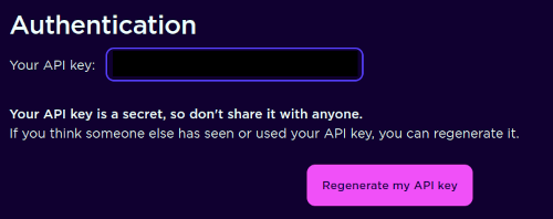
To find your API key, click the link that says Personal details, then find the box labelled Developer settings and click API access

At the top of the screen will be a section labelled Authentication, with your API key just below it

---

Plugin Install

You'll need to have a copy of my plugin on your filesystem. The easiest way to achieve this is to clone my plugins repo (allowing easy access to updates and other plugins)

git clone https://github.com/bentasker/telegraf-plugins.git
sudo mv telegraf-plugins /usr/local/src/

Then, assuming you already have Telegraf installed and configured (if not, see the install instructions), it's just a case of adding configuration so that the plugin is invoked.

Add the following to /etc/telegraf/telegraf.conf:

[[inputs.exec]]
    commands = [
        "/usr/local/src/telegraf-plugins/octopus-energy/octopus-energy.py",
    ]
    timeout = "60s"
    interval = "1h"
    name_suffix = ""
    data_format = "influx"
    # Update the value of these
    environment = [
    "OCTOPUS_KEY=bbbbbaaaaaa",
    "OCTOPUS_ACCOUNT=A-1234567"
    ]

Remember to replace the values for your API key and account number.

Restart Telegraf

systemctl restart telegraf

Telegraf should now poll the Octopus API once hourly.

---

Lag on Consumption Details

Although the plugin will collect consumption data, the values will stop at the end of the previous day.

This is because of the way that smart meter readings are collected: The meter takes a reading every 30 minutes, but stores it locally. The provider then collects those stored reads once a day.

As a result, the readings available via the API always lag behind. This means they're not much use for realtime monitoring (for that you want something more like this), but the values given by the API are what Octopus use to calculate your bill so they're not without, err, value.

---

Timestamps

The timestamp on datapoints for both octopus_pricing and octopus_consumption represent the end of each 30 minute window.

So, if an octopus_consumption point has a time of 10:30 and a value of 1kWh, it indicates that you consumed 1kWh between 10:00 and 10:30.

Pricing data's use of the end of each period is a little less intuitive, but it's structured this way to ensure that the correct price is used when the data is joined to the consumption data.

Timeshifting with Grafana Transforms

Having a pricing period marked by its end time isn't great for human consumption though: we tend to assume it'll start at the given time. However, the timestamp can be corrected in pricing charts by using Grafana Transforms to apply a timeshift (if you're querying with Flux rather than InfluxQL, you could also use timeShift() instead).

If we start with the following InfluxQL query

SELECT
   mean("cost_inc_vat")/100 AS "mean_cost_inc_vat" 
FROM "Systemstats"."autogen"."octopus_pricing" 
WHERE 
   $timeFilter 
   AND "charge_type"='usage-charge' 
   AND tariff_direction != 'EXPORT' 
GROUP BY time(30m)

To apply a timeshift in Grafana we need to

• Calculate a new field called newtime by subtracting 30m (1800000ms) from time (with Add field from calculation)
• Convert oldtime from an integer to a timestamp (with Convert field type)
• Filter Time out of the resultset (with Filter by name)

This works because Grafana is able to treat a Time column as being either a time object or an integer (its integer value being an epoch timestamp), so it's trivial to subtract a fixed period.

Working out how to have Grafana ignore the original time column took a bit longer though.

---

Visualisation

The plugin only creates a few series, so visualisation is quite straightforward.

Consumption details:

SELECT 
   mean("consumption") AS "mean_consumption" 
FROM "Systemstats"."autogen"."octopus_consumption" 
WHERE 
  $timeFilter 
  AND "is_export" != 'True' 
GROUP BY time(30m) FILL(null)

Pricing (using Flux with a timeshift, see above for notes on doing the same with InfluxQL and Grafana transforms)

from(bucket: "Systemstats")
 |> range(start: v.timeRangeStart, stop: v.timeRangeStop)
 |> filter(fn: (r) => r._measurement == "octopus_pricing")
 |> filter(fn: (r) => r._field == "cost_inc_vat")
 |> filter(fn: (r) => r.tariff_direction != "EXPORT")
 |> filter(fn: (r) => r.charge_type == "usage-charge")
 |> keep(columns: ["_time", "_field", "_value", "tariff_code"])
 |> aggregateWindow(every: 30m, fn: mean)
 |> timeShift(duration: -30m)

Calculating Consumption cost over time is a little more complex, with two queries being defined and then joined:

Query A gathers consumption details

SELECT 
  mean("consumption") AS "mean_consumption" 
FROM "Systemstats"."autogen"."octopus_consumption" 
WHERE 
   $timeFilter 
   AND "is_export" !='True' 
GROUP BY time(30m) 

Query B gathers (unshifted) pricing

SELECT
   mean("cost_inc_vat")/100 AS "mean_cost_inc_vat" 
FROM "Systemstats"."autogen"."octopus_pricing" 
WHERE 
   $timeFilter 
   AND "charge_type"='usage-charge' 
   AND tariff_direction != 'EXPORT' 
GROUP BY time(30m) 

Grafana transforms can then be used to join the two and multiply to calculate the cost

The result is a graph showing consumption cost per 30 minutes

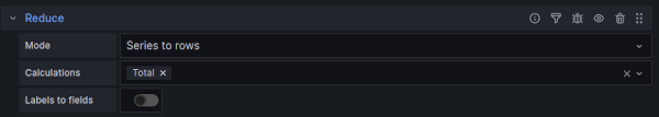
To get the total in-period cost, a second copy of the cell can be made with an additional Reduce transform applied

Exactly the same approaches can be used to calculate export graphs.

The result is a simple, but informative, dashboard

An importable example of this dashboard can be found in my plugins repo.

---

Use in Downsampling & Normalisation

We recently moved from our original energy consumption monitoring to using data collected from our smart meter. In addition to that, we've changed energy supplier and moved onto a variable rate tariff.

These changes made it quite difficult to have a single query show usage/cost over time - the shape of the data changed quite dramatically with each transition, so each stage ended up needing a different query.

This inconsistency also made it very hard to track the savings generated by our Solar install: each solar kWh that we've consumed needs to be tied to the prevailing import cost. Without that information, it's impossible to gauge where we are on the path towards ROI.

So, I decided that, even though the data itself doesn't really need downsampling (it's already at a 30m granularity), it would be worth having a downsampling-like job that could normalise solar savings data into a pricing-source agnostic schema.

My downsampling engine has support for custom queries, so the easiest solution was to write a Flux query capable of pulling the source information in order to generate a provider agnostic output

// Get Octopus pricing
pricing = from(bucket: "Systemstats/autogen")
    |> range(start: v.timeRangeStart, stop: v.timeRangeStop)
    |> filter(fn: (r) => r._measurement == "octopus_pricing" 
        and r._field == "cost_inc_vat"
        and r.charge_type == "usage-charge"
        and r.tariff_direction != "EXPORT"
        )
    |> filter(fn: (r) => r.payment_method == "None")
    |> aggregateWindow(every: 30m, fn: max)
    |> keep(columns: ["_time","_field","_value"])

// Get generation info
solar_yield = from(bucket: "Systemstats/autogen")
    |> range(start: v.timeRangeStart)
    |> filter(fn: (r) => r._measurement == "solar_inverter" 
        and (r._field == "todayYield"
             or r._field == "gridSellToday"
             or r._field == "batteryChargeToday" 
             or r._field == "batterySupplyToday"
        ))
    |> aggregateWindow(every: 30m, fn: max)
    |> difference(nonNegative: true)
    |> keep(columns: ["_time","_field","_value"])
    |> pivot(rowKey: ["_time"], columnKey: ["_field"], valueColumn: "_value")
    |> map(fn: (r) => ({
        _time: r._time,
        // Stuff sold to the grid has a different price
        // energy put into the battery shouldn't be counted as it's
        // value is determined by the price when it's drawn back out
        _value: (r.todayYield - r.gridSellToday - r.batteryChargeToday) + r.batterySupplyToday,
        _field: "available solar yield"
    }))

// Join the two
join(tables: {price: pricing, yield: solar_yield}, on: ["_time"])
    |> map(fn: (r) => ({ 
    _time: r._time,
    // calculate value
    _value: r._value_price * r._value_yield,
    _field: "solar_value_pence",
    _measurement: "solar_value"
    }))

This translates easily into a downsample jobfile:

# Fetch solar yield values along with prevailing
# energy prices to calculate the value of any solar 
# energy that was generated and used or stored 
# (i.e. subtract any export)
downsample_solar_generation_value:
    name: "Downsample Solar generation value"
    influx: home1x
    # Query the last 2 days in case we
    # missed a run
    period: 2880
    # Not used, but needs to be defined
    window: 10
    query: >
        pricing = from(bucket: "Systemstats/autogen")
            |> range(start: v.timeRangeStart, stop: v.timeRangeStop)
            |> filter(fn: (r) => r._measurement == "octopus_pricing" 
                and r._field == "cost_inc_vat"
                and r.charge_type == "usage-charge"
                and r.tariff_direction != "EXPORT"
                )
            |> filter(fn: (r) => r.payment_method == "None")
            |> aggregateWindow(every: 30m, fn: max)
            |> keep(columns: ["_time","_field","_value"])

        solar_yield = from(bucket: "Systemstats/autogen")
            |> range(start: v.timeRangeStart)
            |> filter(fn: (r) => r._measurement == "solar_inverter" 
                and (r._field == "todayYield"
                     or r._field == "gridSellToday"
                     or r._field == "batteryChargeToday" 
                     or r._field == "batterySupplyToday"
                ))
            |> aggregateWindow(every: 30m, fn: max)
            |> difference(nonNegative: true)
            |> keep(columns: ["_time","_field","_value"])
            |> pivot(rowKey: ["_time"], columnKey: ["_field"], valueColumn: "_value")
            |> map(fn: (r) => ({
                _time: r._time,
                _value: (r.todayYield - r.gridSellToday - r.batteryChargeToday) + r.batterySupplyToday,
                _field: "available solar yield"
            }))

        join(tables: {price: pricing, yield: solar_yield}, on: ["_time"])
            |> map(fn: (r) => ({ 
            _time: r._time,
            _value: r._value_price * r._value_yield,
            _field: "solar_value_pence",
            _measurement: "solar_value"
            }))

    aggregates:
        copy:

    output_influx: 
        - influx: home2xreal
    output_bucket: Systemstats/rp_720d

The result is a new measurement called solar_value with a field called solar_value_pence.

I wrote and manually ran similar queries (using to()) to populate historic data, based on whichever pricing source was authoritative at the time.

The availability of this data allowed me to create a dashboard that details the savings that we've made as well as projecting the time remaining until we break even.

The Amortisation Period at Mean Monthly Savings cell is driven by this query

capital_cost = <redacted>

// Calculate the average saving per month since install
monthly_avg = from(bucket: "Systemstats/rp_720d")
  |> range(start: v.timeRangeStart, stop: v.timeRangeStop)
  |> filter(fn: (r) => r["_measurement"] == "solar_value")
  |> filter(fn: (r) => r["_field"] == "solar_value_pence")
  |> aggregateWindow(every: 1mo, fn: sum, createEmpty: false)
  |> keep(columns: ["_field", "_time", "_value"])
  |> mean()
      |> findRecord(
        fn: (key) => true,
        idx: 0,
    )

// Calculate the amount saved to date
saved_td = from(bucket: "Systemstats/rp_720d")
  |> range(start: v.timeRangeStart, stop: v.timeRangeStop)
  |> filter(fn: (r) => r["_measurement"] == "solar_value")
  |> filter(fn: (r) => r["_field"] == "solar_value_pence")
  |> aggregateWindow(every: 1d, fn: sum, createEmpty: false)  
  |> keep(columns: ["_field", "_value"])
  |> sum()


// Subtract the amount saved to date from the capital cost
// then divide the remainder by the average monthly saving
// 
// finally, convert to days for Grafana's benefit
saved_td
  |> map(fn: (r) => ({r with 
     _value: ((capital_cost - (r._value / 100.0)) / 
     (monthly_avg._value / 100.0) * 30.0)
  }))

The result is the estimated number of days until the amount we've saved equals the amount we paid for the install. Obviously the result is fairly rough (and will be skewed by anomalous months), but the result lines up with what I've calculated on paper.

Once our export tariff is up and running, I'll also need to adjust the queries to factor export revenue in (though I'll likely write that into a second field)

---

Conclusion

Octopus's API makes it easy to capture pricing and consumption details with Telegraf.

That data can then be used to monitor energy usage costs as well as to track the savings generated by our solar install (and the benefit of any energy saving experiments that we might try).

In a previous post I wrote

Because we track usage of our appliances, it should also be possible to write a notebook that can consume weather forecasts along with historic generation and weather data in order to (roughly) predict when best to turn appliances like the dishwasher on.

Because Octopus make pricing available in advance, we should actually be able to go one step further and factor grid pricing into the equation (allowing a prediction to still be given for days with adverse weather).

With a little bit of effort, I've been able to create a normalisation job to take data from the various pricing sources I've previously used and write solar savings stats out into a provider agnostic schema. The obvious next step on that, is to do exactly the same thing with unit cost information.